Electromagnetic Radiation Explained

I now dedicate this page in memory of my friend Ron Rackley, who passed away on April 12, 2019. Ron inspired me to further my studies of EM waves and radiation and, ultimately, this page. I will never know as much about radiation as Ron, who devoted his life as a consulting engineer for many radio transmitting facilities all over the world.

There seems to be widespread disagreement about whether the E and H fields propagate in-phase or 90 degrees out of phase. Near the antenna, the dominating field is the Near Field. In this field, the E and H fields are 90 degrees out of phase in time. At a certain point not too far from the antenna, possibly one wave length, exists a transition zone from Near Field to Far Field. After the transition zone the Near Field has faded away (due to a 1/r4 product) and the Far Field becomes the dominant field. The E and H field are in-phase in time in the Far Field and this is the field that is the radiated field to space the impedance of space is said to be about 377 ohms resistive. The E and H field are ALWAYS in a 90 degree spatial relationship to each other. This is not to be confused with the time phase relationship. I am in the process of updating this page to better explain the Far and Near Fields and their transition. I hope this clears up the confusion about the phase relationship of the E and H fields in a radiated signal used for normal, distant communications. Near and Far Field Patterns (Wiki) Want more proof that Electric and Magnetic fields are In Phase? Spend an hour watching a Yale Lecture. Maxwell's Equations and Electromagnetic Waves (Yale Video) see bottom of this page. A bibliography of the books and websites used to support the above information will be added. I am providing a special email address for anyone who wants to make comments, criticisms, suggestions or otherwise, relating to this subject. Send comments to the following address: radiation@j-hawkins.com

One of the least understood phenomena in electrical engineering is the idea that electric and magnetic fields appear to leave a radio transmitting antenna to form what we know as radio waves. Most books fall just short of explaining this process by making statements that fields snap or jump off the antenna as they expand. At the same time, books on electromagnetics present the needed laws of field behavior to explain wave propagation, but are so advanced that it can be difficult for us to relate what we are learning to radiation. This explanation attempts to go beyond the elementary treatments, while at the same time keeping the mathematics a notch simpler than the more advanced treatments of fields. This article will attempt to give the reader a better feel for how electromagnetic fields behave to provide propagated radio signals. My original reference in understanding this topic is a book called Radio-Electronic Transmission Fundamentals by B. Whitfield Griffith, Jr., 1962, re-published in 2000. Additional sources are listed in the bibliography provided at the end of this article. Clarification has been added to explain the in-phase relationship between the two fields as they propagate through space. A knowledge of trigonometry, calculus and vectors is assumed as well as a fairly good background in Electrical Engineering.

A changing magnetic field will create an electric field in space A changing electric field will create a magnetic field in space Definition of radiation and propagation: Explain the transition point between conduction fields around the antenna or radiator to fields in space Show how radio waves propagate via oscillating magnetic fields in space. Radiation Resistance (electronic "friction" and "bootstrap" forces) Bibliography Related Links

The whole is the summation of its parts: The voltage, which is induced in the loop does not arise at any single point in the loop, but, rather is the summation of all the infinitesimal bits of voltage that are arising around the loop, distributed along its contour. If the total distance around the contour of the loop is s, the differential element of length along the contour is said to be ds. Hence, the total voltage induced in the loop will be the dot product , summed or integrated once around the contour of the loop.

	The total voltage around the loop is the sum of all the infinitesimal pieces of voltage around the contour of the loop. Each bit of voltage is represented by the dot product of the electric field intensity volts/meter and the segment length. (The field component, which is tangent to the loop at that point.)
Eq. 1

Now, we find the relationship of the total voltage to the magnetic flux density B. Faraday's Law - The voltage induced in a loop of wire is directly proportional to the rate of change of the magnetic flux which links or passes through that loop.

	In other words, it is the time derivative of the flux linkage.
Eq. 2

Since, according to Faraday's law, this total voltage is solely dependent on the rate of change of the total flux , passing through the loop, it is important to know how the total flux is related to the density of the magnetic flux.

	The differential flux is the dot product of the flux density with the unit vector normal (perpendicular to) the differential area, which says that it is the component of flux which is passing perpendicularly through the element area da.
Eq. 3

The total flux can now be expressed in terms of the flux density as follows:

	To obtain the total flux passing through the contour area, we sum the differential pieces by integrating both sides of the equation.
Eq. 4

Recalling Faraday's law, stating that the voltage induced in the loop is proportional to the rate of change of the flux, we can differentiate the above integral with respect to time to get the voltage as related to the flux.

Eq. 5

Getting back to Faraday's law, if we were to hold up a ring of wire in front of us and have an expanding (increasing positively) magnetic flux passing through it, but away from us, the induced voltage would cause a current flow in a counterclockwise direction. The counterclockwise current flow, is contrary to the right-hand screw rule, therefore we consider it a negative flow. Following this, Faraday's law equation is rewritten as follows:

Eq. 6

Now, substituting each side of Eq. 6 with Eq. 1 on the left side and Eq. 5 on the right side, yields the first of the field equations as shown in Eq. 7.

Eq. 7

The circle added to the integral symbol indicates that we are integrating around the entire closed contour. This provides a means of computing the induced voltage in a loop of arbitrary size and shape with any distribution of magnetic flux within the enclosed area. The most important implication of this equation is that it relates an electric field with a changing magnetic flux without considering that any current carrying wire is present. In other words, electric fields can exist in space without a conductor, allowing for energy to be transferred from one place to another without a physical conductive connection.

Correction from previous statement here: This statement says that the induced voltage in a closed loop, which is the CURL in space, is proportional to the change in magnetic flux with respect to time. The CURL actually represents the electric field at a point of maximum change in space. This puts the two orthogonal waves IN PHASE, because the maximum CURL (minimum amplitude of E), occurs at a point of minimum amplitude of the magnetic field. The relationship of the CURL to a line integral of a closed path is proven by Green's Theorem. A full understanding of Green's theorem, line integrals and curls are subjects of higher level of Calculus. If one desires a better understanding of these concepts I would recommend the sequence of lessons given online by Sal Khan of Khan's Academy. If you already know two dimensional calculus and vector operations, such as the cross product and dot product, you should be able to extend your knowledge in a relatively short period of time. Khan Academy sequence of line integrals and Green's Theorem can be found at the following link: https://www.khanacademy.org/math/calculus/line_integrals_topic Or by searching YouTube

---

A changing electric field will
create a magnetic field in space.

Biot-Savart law - If a long, straight conductor carrying a current, it will cause a magnetic field of intensity H to surround it at any radial distance r, hence the Biot-Savart Law equation:

Eq. 8

We can obtain the magnetomotive force with a relation that is analogous to that used to obtain the electromotive force as expressed in Eq. 2.

	The total magnitomotive force is the sum of the components of magnetic field strength tangent to the contour.
Eq. 9

If we assume that the conductor is long and straight and passes perpendicularly through the center of the contour, the solution simplifies to:

Eq. 10

Substituting equation 8 and the circumference of a circle for H and s respectively give us:

Eq. 11

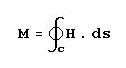
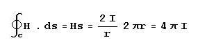
Note that the radius has been canceled in the equation, which means that the magnetomotive force around the contour is independent of the radius or, for that matter, even the shape of the contour. A circle is the special case where r is constant in a curve expressed in polar coordinates and that a non-circle is when r is a function of the angle. So, whether r is constant or variable with the angle, the total magnetomotive force is dependent only on the current through the conductor. 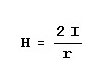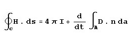This equation tells us that a current passing through a conductor results in a magnetic field and that the strength of the magnetic field is proportional to the current. It follows that if the magnitude of the current were varying in any way, the resultant magnetic field would also vary. So, if the current were alternating in a sinusoidal fashion at some frequency, the magnetic field would also be caused to alternate at the same frequency. 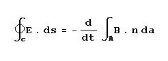So far we have shown that an alternating current through a wire or conductor results in alternating magnetic and electric fields around the conductor. So far, we have not shown that these fields radiate or "leave" the conductor on a distant journey in any way nor do they "snap," "jump," or "hop" off the antenna as many texts would have you believe. In order for radiation to be able to occur, we have to prove that magnetic and electric fields can exist without the presence of a nearby current and that these fields will "move" through space. We will see the idea of movement of these fields through space as radio waves is really an abstraction. What really happens is more of a domino effect, which is a demonstration of "propagation." In order to begin to understand the transition between the fields we have just described, which are referred to as conduction fields and fields that become free of the wire we must find some way to relate what happens in a conductor to what happens in space. We will start off by stating Kirchoff's law. 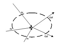Kirchoff's Law - The sum of all currents entering and leaving a node or branch point in a circuit must equal zero as illustrated by figure 1..

Fig. 1

Expanding this to an enclosed volume. If the dashed line in Fig. 1 represents an enclosed volume then, the sum of all the currents entering the boundary of the volume must equal the sum of all the currents passing out of the volume. Mathematically speaking, the integral of the current density over the entire volume regardless of shape or size equals zero. Current cannot be dead ended inside of a volume. What goes in, must come out. Let us now enclose one of the plates of a capacitor with a volume as shown in Fig. 2.

Fig. 2

The boundary of the volume passes between the plates. The arrows indicate a current entering the left capacitor lead and exiting the right capacitor lead. Since there is no conductive connection between the plates, how can we apply Kirchoff's law if current cannot actually flow out of the volume enclosed by the dotted line to get to the right capacitor plate? The answer lies in the idea of displacement current.

Displacement Current - First, we introduce dielectric displacement. The dielectric displacement, designated by the letter D, represents the electrical strain which occurs in a dielectric medium, when an electric field is present.

	D is analogous to magnetic flux density B, hence D is really the electric flux density. It is related to the electric field by , which is the permittivity or dielectric constant of the material between the plates of a capacitor. The magnetic flux density B is related to the magnetic field strength H by or the permeability of the material within the magnetic field.
Eq. 12a and 12b

To explain what is happening between the plates of the capacitor, we first realize that as current flows into the capacitor, an electric charge accumulates on the plates with excess electrons on one plate and a dearth of them on the other. As the charge builds up, an electric E field between the plates, builds up causing the dielectric displacement or electric field density to also increase. In order to satisfy Kirchoff's law, there must be some sort of current flowing in the dielectric, proportional to the rate of change of dielectric displacement. This current has been given the name displacement current and we can think of it as a flowing-in (displacement) of additional flux as required as the electric flux density increases. This total displacement current is equal to the conduction current flowing into and out of the capacitor and, therefore, out of the volume with which we have surrounded the plate. As Maxwell was aware of the displacement current, he had to decide whether it was consistent with conduction current in that it would also have a magnetic field associated with it. Maxwell, then made the assumption that there was, indeed a magnetic field associated with the displacement current. In considering this, he added an additional term into the of Ampere's Rule and the Biot-Savart equation to account for it. Equation 13 shows this new relationship.

Eq. 13

This equation takes into consideration that the area within the contour of H . ds integration might contain both conduction and displacement currents which would both contribute to the intensity of a magnetic field. D . n da is the differential electric flux across the capacitor space normal to a given point and the integral sums it up to the total flux. The rate of change of the total flux is the displacement current flowing through the contour.

	A changing magnetic field normal to a closed surface is proportional to the curl of the electric field around a closed loop.
	A changing electric field normal to a closed surface is proportional to the curl of the magnetic field, around a closed loop.
Eq. 14 and 15 Maxwell's free space equations.

If we make the appropriate substitutions from Eqs. 12a and 12b to Eq. 14 and 15, we have:

	Where Mu is the permiability of free space (it should be Mu Naught).
	Where Epsilon is the permittivity of free space (it should be Epsilon Naught).
Eq. 16 and 17 Maxwell's free space induction equations. Faraday's Law in integral form.

E and B relationships can easily be satisfied with the differential
form of the Maxwell Faraday Equation.

	Differential form of Faraday's Law relating E to B fields in space.
	With: E field amplitude in x along Z axis B field amplitude in y along Z axis Both equations are expressed as vectors along the unit vectors i, j, k axes.
	Plugging E and B into Faraday's Law, the solutions is true for the phase difference of zero and k = w.
Eq. 18, 19 and 20: Maxwell's free space equations. Faraday's Law says that the curl of the induced electric field is equal to the time rate of change of the magnetic field. The two fields are physically orthogonal or perpendicular in space and they are in phase with each other. OR - The spatial variation of the electric field, E, gives rise to a time-varying magnetic field, B, and visa-versa. Professor Ramamurti Shanker of Yale University proves out the radiated wave using the differential form of Maxwell's Equation which is Faraday's Law. See embedded YouTube video below. The ratio of the magnetude of the E field to the B field is equal to the speed of light 'c'. That is, the magnetude of the magnetic wave is only 3*(10-8) of the amplitude of the electric wave! (Still more details and a full derivation to come!) See Also: 1) Wave Equation Derivation by Lynda Williams, Santa Rosa Junior College Physics Department 2) Maxwell's Equations and Electromagnetic Waves - MIT study guide chapter 13

These equations are the key to electromagnetic radiation! Most important is the fact that no conduction current need exist and, therefore, no physical conductor.

---

Bibliography

Advanced Calculus, Wilfred Kaplan, 5th Printing, Addison Wesley, 1959 "div grad curl and all that", H. M. Schey, 3rd edition, Norton 1997 Electromagnetics, John D. Kraus, Fourth Edition, McGraw Hill, 1992 Engineering Electromagnetics, William H. Hayt, Jr., 5th Ed., McGraw Hill, 1989 Radio-Electronic Transmission Fundamentals, B. Whitfield Griffith, Jr., 1962, re-published in 2000. University Physics, Sears and Zemansky, 3rd Edition - Complete, Addison Wesley, 1964 "Why an Antenna Radiates" by Dr. Kenneth MacLeish, QST magazine.

Accessed

times since August 2, 2000.

WIKI Electromagnetic Radiation Electromagnetic Radiation (The Mysearch Website) Understanding electromagnetic fields and antenna radiation takes almost no math ARRL Technical Information Service: Why an Antenna Radiates by Kenneth Macleish Eric Weisstein's World of Physics Georgia State University - Index to Hyperphysics PHYSICS FORUMS